

Let’s say you want to measure the relationship between multiple variables. One of the simplest ways to do this is through linear regression (e.g. ordinary least squares). However, this methodology assumes that the relationship between all variables is linear. One could also use generalized linear models (GLM) in which the variables are transformed, but again the relationship between the outcome and the transformed variable is (you guessed it) linear. What if you wanted to model the following relationship?
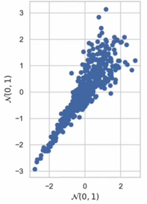
In these data, both variables are normally distributed with a mean of 0 and a standard deviation of 1. Furthermore, the relationship is largely comonotonic (that is, as variable x increases so does y). However, the correlation is not constant; The variables are closely correlated for small values, but weakly correlated for large values.
Does this relationship really exist in the real world? It certainly is so. In financial markets, the returns of two different stocks may have a weakly positive relationship when the stocks rise; However, during a financial crisis (e.g. COVID, dotcom bubble, mortgage crisis), all stocks go down and therefore the correlation would be very strong. Therefore, it is very useful that the dependence of different variables varies depending on the values of a given variable.
How could you model this type of dependency? TO great series of videos by Kiran Karra explains how copulas can be used to estimate these more complex relationships. To a large extent, copulas are constructed using Sklar’s theorem.
Sklar’s theorem states that any multivariate joint distribution can be written in univariate terms marginal distribution functions and a copula that describes the dependency structure between the variables.
https://en.wikipedia.org/wiki/Copula_(probability_theory)
Copulas are popular in high-dimensional statistical applications, as they allow the distribution of random vectors to be easily modeled and estimated by estimating marginals and copulas separately.
Each variable of interest is transformed into a variable with a uniform distribution ranging from 0 to 1. In Karra’s videos, the variables of interest are x and and and the uniform distributions are you and v. Using Sklar’s theorem, you can transform these uniform distributions into any distribution of interest using an inverse cumulative density function (which are the functions F-inverse and GRAM-inverse respectively.
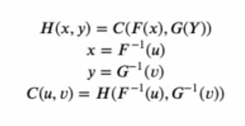
Essentially, the variables from 0 to 1 (u,v) serve to rank the values (i.e., percentiles). So if u=0.1, this gives the 10th percentile value; if u=0.25, this gives the 25th percentile value. What the inverse CDF functions do is, if you say u=0.25, the inverse CDF function will give you the expected value for x at the 25th percentile. In summary, while the math seems complicated, in reality we can only use marginal distributions based on values ranked 0.1. More information about the mathematics behind copulas is below.
The next question is, how do we estimate copulas with data? There are two key steps to doing this. First, you need to determine which copula to use, and second, you need to find the copula parameter that best fits the data. In essence, copulas aim to find the underlying dependent structure (where the dependence is based on ranks) and the marginal distributions of the individual variables.
To do this, first transform the variables of interest into ranges (basically, changing x,y in u,v in the previous example). Below is a simple example where continuous variables are transformed into range variables. To increase the variables u,v, simply divide by the maximum range + 1 to ensure that the values are strictly between 0 and 1.
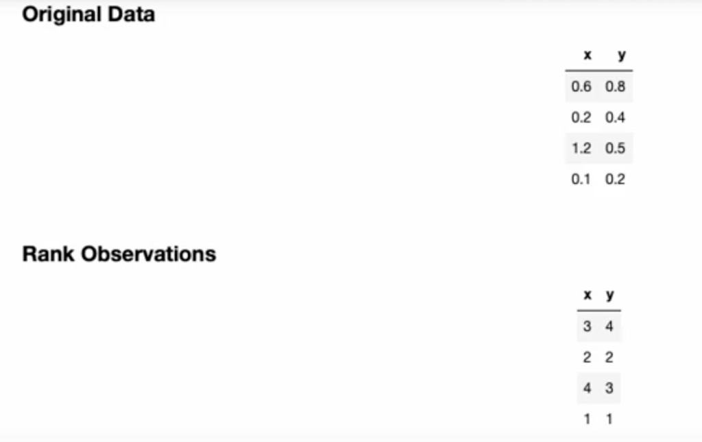
Once we have the range, we can estimate the relationship using Kendall’s Tau (also known as Kendall rank correlation coefficient). Why would we want to use Kendall’s Tau instead of a regular correlation? The reason is that Kendall’s Tau measures the relationship between ranks. Therefore, Kendall’s Tau is identical for the original and classified data (or, conversely, identical for any inverse CDF used for the marginals conditional on a relationship between u and v). In contrast, the Pearson correlation can vary between the original and classified data.
Then you can choose a form of copulation. Common copulas include the Gaussian, Clayton, Gumbel, and Frank copulas.
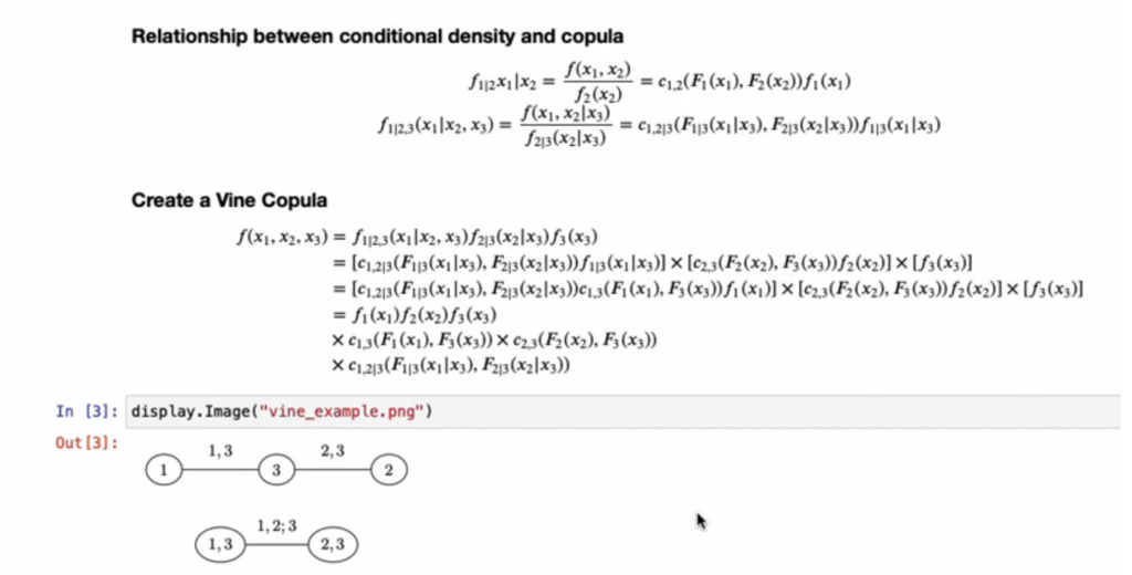
The previous example was for two variables, but an advantage of copulas is that they can be used with multiple variables. Computing joint probability distributions for a large number of variables is often difficult. Therefore, one way to arrive at statistical inference with multiple variables is to use vine copulas. Vine copulas are based on chains (or vines) or conditional marginal distributions. In summary, an estimate
For example, in the following 3-variable example, the joint distributions of variable 1 and variable 3 are estimated; the joint distribution of variable 2 and variable 3 and then the distribution of variable 1 conditional on variable 3 can be estimated with variable 2 conditional on variable 3. While this seems complex, in essence, we are doing a series of pairwise joint distributions rather than trying to estimate joint distributions based on 3 (or more) variables simultaneously.
The following video describes vine copulas and how they can be used to estimate relationships for more than 2 variables using copulas.
For more details, I recommend seeing the a whole series of videos.


